
Static mixer formulas
The textbook relations behind static mixer sizing, what they tell you, and where supplier data has to take over from the formulas.
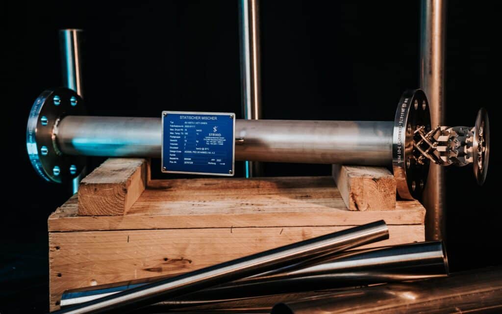
The key static mixer formulas are the Reynolds number, which sets the flow regime, the pressure drop relation, often written as a multiple of the empty pipe pressure drop, and the mixing relation, in which the coefficient of variation falls with every element. Their general form is well established, but the constants depend on the element design. A reliable sizing therefore needs the manufacturer’s own data.
- Why static mixer formulas matter before you talk to a supplier
- Static mixer formulas start with the Reynolds number
- Pressure drop: from empty pipe to mixer
- Mixing length: elements, layers and the coefficient of variation
- An indicative walk-through of the static mixer formulas
- Where textbook static mixer formulas stop
- How we size a static mixer with you
Unsure about the right choice?
Share your process data with our specialists. We check the numbers with you and give reasoned advice.
Why static mixer formulas matter before you talk to a supplier
Static mixer formulas are where process engineering gets honest about a piece of equipment that has no moving parts and no motor, yet still has to deliver a measurable result. A static mixer takes its mixing energy from the pressure drop in the line. Every element that splits, redirects and recombines the flow costs a little pressure and buys a little homogeneity. The formulas describe that trade: how much mixing you get, over what length, for what pressure loss.
At Dutch Valve Vision we size STRIKO static mixers together with our customers, as the exclusive agent of STRIKO Verfahrenstechnik GmbH for the Netherlands, Belgium and Luxembourg. We welcome it when an engineer arrives with a rough calculation of their own. The conversation then starts from physics rather than from a catalogue page, and unrealistic expectations surface early, such as a very short mixer with hardly any pressure drop for a highly viscous additive.
This page walks through the static mixer formulas found in most textbooks on mixing and fluid flow: the Reynolds number, the pressure drop relations and the way mixing quality develops along the mixer. Please read every relation here as indicative. The general form is well established, but the constants that make the equations useful belong to a specific element design and come from the manufacturer’s test data. We return to that point at the end, because it is the reason a supplier sizing remains necessary.
Static mixer formulas start with the Reynolds number
Every calculation begins with the flow regime, and the flow regime begins with the Reynolds number. For a pipe it is defined as Re = ρ × v × D / μ, where ρ is the density, v the mean velocity in the empty pipe, D the internal pipe diameter and μ the dynamic viscosity. The result is dimensionless. It expresses the ratio between inertial forces, which tend to create eddies, and viscous forces, which tend to damp them.
Two quick examples show why it matters. Water at around room temperature has a density of about 1000 kg/m³ and a viscosity of about 0.001 Pa·s. In a pipe with an internal diameter of roughly 0.05 m and a velocity of 1 m/s, that gives Re = 1000 × 1 × 0.05 / 0.001 = 50,000, which is clearly turbulent. Now replace the water with a viscous liquid of 10 Pa·s, in the same pipe, at the same velocity and a similar density. The Reynolds number drops to 5. Same pipe, same velocity, and a completely different mixing problem.
In an empty pipe, the textbook transition from laminar to turbulent flow lies at a Reynolds number of around 2300. Inside a static mixer that boundary shifts, because the elements disturb the flow and turbulence sets in earlier. Where exactly depends on the element geometry, which is why manufacturers define laminar, transitional and turbulent ranges for each of their own designs. The practical rule is simple: calculate Re with the empty pipe diameter and velocity, then check which regime that places you in for the specific mixer type.
The regime matters because the mixing mechanism changes. In laminar flow, the elements do the work by cutting and folding the stream into ever thinner layers. In turbulent flow, the elements generate additional eddies and mixing is driven by turbulent dispersion. The pressure drop and mixing length relations change accordingly, and so does the right choice of mixer.

Pressure drop: from empty pipe to mixer
The static mixer formulas for pressure drop start from the empty pipe. The Darcy-Weisbach equation gives Δp = f × (L / D) × (ρ × v² / 2), where f is the Darcy friction factor and L the pipe length. In laminar flow the friction factor follows directly from theory as f = 64 / Re. Substituting that shows that laminar pressure drop is proportional to viscosity, velocity and length, and inversely proportional to the square of the diameter.
A static mixer adds resistance on top of that. The simplest way to express it is the Z factor, where the pressure drop over the mixer equals Z times the pressure drop over an empty pipe of the same length and diameter. In laminar flow Z is roughly constant for a given element design, while in turbulent flow it changes with the Reynolds number. Another common form uses the Newton number, Ne = Δp × D / (ρ × v² × L), a dimensionless pressure drop per unit length. In the laminar regime the product Ne × Re tends towards a constant for each element type, whereas in the turbulent regime Ne itself levels off.
Those relations lead to a few rules of thumb every engineer should keep in mind. In laminar flow at a fixed volume flow, halving the pipe diameter raises the velocity by a factor of four and the pressure drop by roughly a factor of sixteen, because pressure drop then scales with the flow rate divided by the fourth power of the diameter. Doubling the viscosity doubles the pressure drop. In turbulent flow the pressure drop scales roughly with the square of the velocity, so extra throughput is paid for quickly.
The Z factor and Newton number constants are exactly the values that separate one mixer design from another. Published literature gives values for several element types, but they vary with geometry, the number of elements and the way the tests were carried out. For a real design, the manufacturer’s own data for its own element is the only reliable basis.
Mixing length: elements, layers and the coefficient of variation
How long does a static mixer have to be? The answer depends on how you measure mixing quality and on the regime you are in.
In laminar flow with helical elements, the classic idealisation is striation counting. Each element divides the stream in two, so after n elements the number of layers is S = 2^n. The layer thickness shrinks accordingly, to roughly D / 2^n. Ten elements already produce more than a thousand layers, twenty more than a million. Once the layers are thin enough, molecular diffusion completes the mixing in a short time. This simple picture explains why a modest number of elements can homogenise even viscous media, and why the number of elements, not just the length, is the real design variable.
Engineers usually express mixing quality as the coefficient of variation, CoV = σ / x̄, the standard deviation of the concentration across the pipe cross section divided by its mean. A perfectly mixed stream has a CoV of zero. At the inlet, before any mixing, the CoV of an additive injected as a volume fraction φ into the main stream is CoV0 = √((1 – φ) / φ). Small additive fractions therefore start from a high CoV, which is why dosing a small amount of chemical into a large flow is a harder mixing task than blending two streams of similar size.
Along the mixer, the CoV falls roughly exponentially with the number of elements, following CoV / CoV0 = K^n, where K is a constant smaller than one that characterises the element type in a given regime. Rearranged, the number of elements needed to reach a target becomes n = ln(CoV target / CoV0) / ln(K). The target itself comes from the process. A dosing step in water treatment and a colour blend in a consumer product can call for very different levels of homogeneity. Mixer length then follows as the number of elements multiplied by the element length, which manufacturers usually express as a ratio to the pipe diameter.
In turbulent flow the same logic applies, but K takes a different value and mixing length is often expressed in pipe diameters. An empty pipe also mixes in turbulent flow, only slowly, and the mixer’s job is to reach the target over a much shorter distance. These are the static mixer formulas that turn a mixing requirement into a number of elements and a length.
Selection on viscosity, flows, temperature, pressure
Mixing energy comes from the pressure drop
STX series for viscous, syrupy liquids
Validation with pressure test and measuring points
An indicative walk-through of the static mixer formulas
Picture a process engineer at a chemical plant who has to dose an additive into a product line. The additive is a small fraction of the main stream and considerably more viscous. The engineer has the flow rates, the pipe size and the viscosities, and wants a first impression before contacting suppliers.
The first step is the Reynolds number, calculated with the empty pipe diameter, the mean velocity and the viscosity of the main stream. That places the duty in the laminar, transitional or turbulent range for the mixer type under consideration. The second step is the starting point for mixing: with the volume fraction of the additive, the relation for CoV0 gives the inlet coefficient of variation. The third step is the target CoV that the downstream process needs. The fourth step uses CoV / CoV0 = K^n to estimate the number of elements, with a K value from literature or, better, from the manufacturer. The fifth step multiplies that number by the element length to obtain the mixer length. The sixth step applies the Z factor or Newton number to estimate the pressure drop, which the engineer then compares with what the pump and the line can accept.
The outcome is useful, but only as an estimate. The engineer now knows whether the duty is laminar or turbulent, whether the mixer is likely to be long or short, and whether pressure drop may become a constraint. What the engineer does not yet have is a design that can be relied on, because every constant in the calculation belongs to a specific element and was measured under specific conditions. Working through the static mixer formulas in this way is nevertheless the best possible preparation for a sizing conversation.
Where textbook static mixer formulas stop
Real processes rarely match the assumptions behind the textbook. Many products are non-Newtonian, so their viscosity changes with shear rate and the Reynolds number is no longer a single value. The viscosity ratio between additive and main stream has a strong influence on how easily a viscous component is broken up and distributed. Temperature changes the viscosity along the line, sometimes considerably. Gas mixing, gas-in-liquid dissolution, emulsions and heat transfer tasks each bring their own relations and their own uncertainties.
This is where supplier sizing takes over from the static mixer formulas. STRIKO specialises in static mixers for (highly) viscous media, and its range has four series: the EREstat for food and hygienic processes, the Helical as the universal mixer, the STV for gases and the STX for viscous, thick and syrupy liquids. Each has its own element geometry and therefore its own constants. Selecting the right one starts with a proper process analysis of the viscosity of the components, the volume flows, the temperature and pressure, and the required mixing quality.
Validation closes the loop. For a static mixer that has to perform in a critical process, the engineering does not end with the calculation. It includes a pressure test and leak detection, measuring points to check mixing quality in operation, and simulations of flow velocities and homogeneity. Those steps confirm that the mixer delivers in the plant what the formulas predicted on paper.
How we size a static mixer with you
When you send us a sizing request, we work through the same chain as the relations above, using STRIKO’s own data for the element types in question. We start from the viscosities, flow rates, temperatures, pressures and required mixing quality, establish the regime, and select the series, the number of elements, the diameter and the length. We compare the pressure drop with what your line can accept. We also look at materials such as SS316, 1.4404 or 1.4571, carbon steel, PVC, PE or PVDF, and at cleaning requirements, including easy dismantling and, where needed, inline sterilisation and steam cleaning.
Our support does not stop at the calculation. We can look at the mixer together with the valves, measuring instruments and process automation around it, and support installation, validation and optimisation once it is in the line.
If you have done your own estimate with static mixer formulas, send it along. It helps us understand your assumptions, and we will tell you where our figures differ and why. Send your data to sales@dutchvalvevision.com or call +31 (0)70-2210560, Monday to Friday from 09:00 to 17:00. We work under an ISO 9001 certified quality management system, certified by KIWA.
Specification ready? We will prepare a targeted quote.
Send us medium, pressure, temperature and connection. Our specialists come back with a matching proposal.
Frequently asked questions about static mixer formulas
Question not listed? Our specialists are happy to help.
What is the most important formula for sizing a static mixer?
The Reynolds number is the first and most important one. It is calculated as Re = ρ × v × D / μ, using density, mean velocity, pipe diameter and dynamic viscosity. The result tells you whether the flow is laminar, transitional or turbulent. That regime decides which mixing mechanism dominates and which pressure drop relation applies. In an empty pipe the textbook transition lies at a Reynolds number of around 2300. Inside a static mixer turbulence sets in earlier, and the exact boundaries depend on the element design. Every other calculation, from pressure drop to mixing length, builds on this first step. Getting the viscosity right at the actual operating temperature is therefore essential.
How do I calculate the pressure drop of a static mixer?
A common approach starts with the pressure drop of an empty pipe of the same length and diameter. The Darcy-Weisbach equation gives that value, with the friction factor f = 64 / Re in laminar flow. The mixer’s pressure drop is then expressed as Z times the empty pipe value. In laminar flow the Z factor is roughly constant for a given element design. An alternative uses the Newton number, a dimensionless pressure drop per unit length. For laminar flow the product of Newton number and Reynolds number tends towards a constant per element type. These constants come from test data and differ between designs and manufacturers. For a figure you can rely on, the supplier has to calculate the pressure drop with the data for its own elements.
How many mixing elements does a static mixer need?
The number of elements follows from the mixing quality you need and the regime you are in. Mixing quality is usually expressed as the coefficient of variation, the standard deviation of concentration divided by its mean. Along the mixer the coefficient of variation falls roughly as K to the power n, where n is the number of elements. The constant K depends on the element design and the flow regime. Rearranging that relation gives the number of elements needed to reach a target value. In laminar helical mixers the idealised number of layers doubles with every element. The mixer length is then the number of elements multiplied by the element length. We calculate this with STRIKO’s own data when we size a mixer for you.
Why does a small additive fraction make mixing harder?
The starting point of the mixing task depends on the volume fraction of the additive. Before mixing, the coefficient of variation equals the square root of one minus the fraction, divided by the fraction. A small fraction therefore gives a high starting value. The mixer has to bring that value down to the process target, which takes more elements. That is why dosing a small amount of chemical into a large flow is demanding. Where and how the additive is injected also influences the result. Viscosity differences between additive and main stream can make the task harder still. A proper sizing takes all of these factors into account together.
How does viscosity affect static mixer sizing?
Viscosity is often the most influential property in the whole calculation. It appears in the Reynolds number and therefore decides the flow regime. In laminar flow the pressure drop rises in direct proportion to viscosity. A viscous additive in a thin main stream is also harder to break up and distribute. Many products are non-Newtonian, so their viscosity changes with shear rate. Temperature changes viscosity along the line as well. STRIKO specialises in static mixers for (highly) viscous media and offers the STX for thick and syrupy liquids. Always give us viscosity data at the actual operating temperature, and for non-Newtonian products the flow behaviour as well.
Can I size a static mixer myself with textbook formulas?
You can make a useful first estimate, but not a final design. Textbook relations give the general form of the Reynolds number, pressure drop and mixing length. The constants that make those relations work, such as the Z factor or the K value, are specific to each element design. Published values vary with geometry and test conditions. Real fluids add complications such as non-Newtonian behaviour and large viscosity ratios. An own estimate is still valuable, because it shows early whether pressure drop or length will be a constraint. Send it to us along with your process data. We will compare it with the sizing based on STRIKO’s data and explain any differences.
What is the difference between laminar and turbulent static mixing?
In laminar flow the fluid moves in orderly layers and hardly mixes by itself. The elements create the mixing by repeatedly splitting, turning and recombining the stream. This typically applies to viscous media or low velocities. In turbulent flow the elements generate additional eddies that distribute the components quickly. That applies to low viscosity media at higher velocities. The pressure drop behaves differently as well, rising in proportion to velocity in laminar flow and roughly with velocity squared in turbulent flow. The number of elements and the mixer length needed also differ between the two regimes. That is why the regime is always the first thing we establish.
How is a static mixer's performance validated after installation?
Validation starts with a pressure test and leak detection of the mixer section. Measuring points for mixing quality allow homogeneity to be checked in operation. Samples taken downstream can confirm that the coefficient of variation meets the target. Simulations of flow velocities and homogeneity support the design before and after installation. Where the pressure drop is critical, measuring it across the mixer confirms the calculation. Together these steps show whether the mixer delivers what the formulas predicted. We support installation, validation and optimisation of the static mixers we supply. If the process changes later, we can review the sizing with you.
Have your static mixer sized on STRIKO data
Send us the viscosities, flow rates, temperature, pressure, pipe size and target mixing quality, plus your own estimate if you made one. We size the STRIKO mixer and explain any differences.
- +31 (0)70-2210560
- sales@dutchvalvevision.com
- Vlotlaan 641, 2681 TZ Monster, the Netherlands
- Mon-Fri 09:00-17:00